Google Sheet Chart Guide

---

Step One

Create a Chart

1. Go to Google Sheets and create your sheet
   • If you’re not signed in, follow the steps presented to sign in
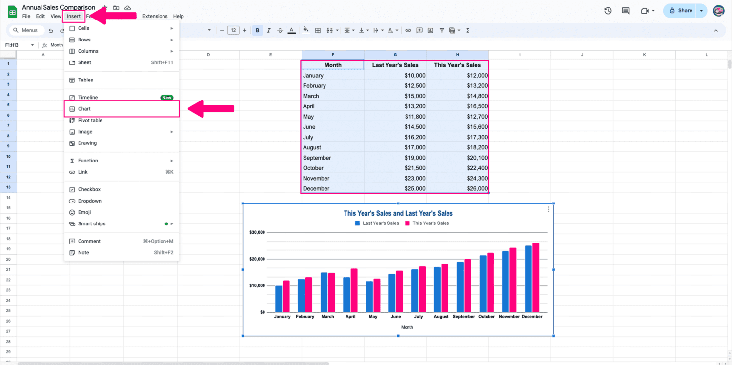
2. Select all the cells you want to include in your chart
3. Click “Insert”, then “Chart”

---

Step Two

Customize Your Chart

Now that you have your chart, select it by double-clicking on it and customize it using the Google Sheets Chart Editor on the right side of your screen.

---

Step Three

Publish Your Chart

With your chart customized to your liking, we can now embed it.

1. Click “File” on the left side of your screen
2. Click “Share”
3. Click “Publish to web”

---

Step Four

Get and Copy the Correct Embed Code

1. Click “Embed”
2. Select your chart instead of “Entire Spreadsheet”
3. Change “Interactive” to “Image”
4. Click the green “Publish” button
5. Copy the entire embed code
   • (Mac: “Command + C”, Windows: “Control + C”)

---

Step Five

Paste the Embed Code into the Google Sheets Chart Slide

1. Paste the copied embed code into the “Google Sheet Chart Embed Code” field in the Google Sheets Chart Retriever slide
   • (Mac: “Command + V”, Windows: “Control + V”)